The Mathematics of Coordinate Transformations
The outline of an organism is drawn onto a system of cartesian coordinates. This figure is therefore treated as a function of x and y. If the rectangular system is altered, for example, by changing the direction of the axes, the ratio x/y or substituting x or y for more complicated expressions, then we obtain a new coordinate system. The outline of the figure will follow this deformation.
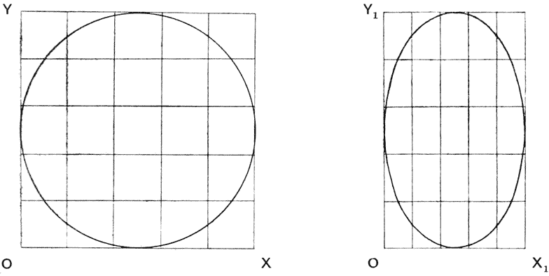
If we take a square grid and extend it along one axis (take the y-axis for example), each little square will become oblong in shape. The original x and y now become x1 and cy1. This transforms the equation of the circle: x2 + y2 = a2 to the equation of an ellipse: x12+c2y12=a2
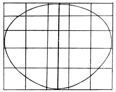
We can also perform a transformation where the extension of an axis is not equal at all distances. Here, for example, the y axis increases logarithmically and y is substituted by ey.
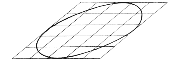
Rectangular coordinates can also become oblique. This is where their axes are inclined to one another at certain angles. x = ε - η cot ω and y = η cosec ω represent an example of new coordinates in an oblique transformation.
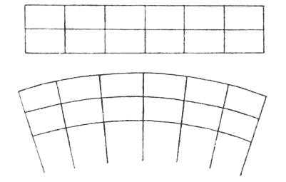
Radial coordinates can also be used. This is where one set of lines are represented as radiating from a point and the other set are transformed into circular arcs. This type of transformation is especially applicable to cases where there exists some part which suffers no deformation (e.g. a node where no growth occurs).
Types of Coordinate Transformations:
(1)
If we take a square grid and extend it along one axis (take the y-axis for example), each little square will become oblong in shape. The original x and y now become x1 and cy1. This transforms the equation of the circle: x2 + y2 = a2 to the equation of an ellipse: x12+c2y12=a2
|
(2)
We can also perform a transformation where the extension of an axis is not equal at all distances. Here, for example, the y axis increases logarithmically and y is substituted by ey.
|
(3)
Rectangular coordinates can also become oblique. This is where their axes are inclined to one another at certain angles. x = ε - η cot ω and y = η cosec ω represent an example of new coordinates in an oblique transformation.
|
(4)
Radial coordinates can also be used. This is where one set of lines are represented as radiating from a point and the other set are transformed into circular arcs. This type of transformation is especially applicable to cases where there exists some part which suffers no deformation (e.g. a node where no growth occurs).
|
In On Growth and Form, D'Arcy gives many examples using the theory of transformations. The four grid transformations above are the most simple cases. D'Arcy combines some of these and uses more complicated transformations in his examples.
Back to the Transformations
Eric Harold Neville
John Marshall
Alfred North Whitehead