Earliest Uses of Symbols for Matrices and Vectors
For matrix and vector entries on the Words pages, see here for a list. For vector analysis words see here; vector analysis symbols are on the calculus page.
Most of the basic notation for matrices and vectors in use today was available by the early 20th century. Its development is traced in volume 2 of Florian Cajori's History of Mathematical Notations published in 1929. Cajori made much use of Thomas Muir's 4-volume The Theory of Determinants in the Historical Order of Development (1906-24) which covered the years 1890-1900; a supplement (1930) brought the story up to 1920.
The modern reader of Muir will be struck that he invested so much in a history of determinants but determinants seemed so much more central at the end of the 19th century when Muir began work than they do now. The modern reader of Cajori will be struck by how very differently the material was organised and the emphasis distributed in his time. Thus matrices appear in a sub-section of "Determinant notations" and vectors in "Symbolism for imaginaries and vector analysis." Muir's investment and Cajori's organisation reflect how the subject(s) developed. The emerging field of abstract linear spaces is hardly noticed by Cajori.
The emphasis on matrices and the blending of matrix algebra and abstract linear spaces only became features of undergraduate mathematics after the Second World War. See the entry LINEAR ALGEBRA on Words.
These developments can be followed in the general histories, e.g.,
- Morris Kline Mathematical Thought from Ancient to Modern Times. Oxford University Press, 1972.
- Victor J. Katz, A History of Mathematics: An Introduction. Harper Collins, 1993, or Addison Wesley, 1998
Notation for Systems of Linear Equations
The modern notation for systems of linear equations did not become established until the early twentieth century, though by then such systems had been studied continuously in the West for perhaps 200 years. MacTutor: Matrices and determinants describes how GAUSSIAN ELIMINATION (see below) was known to Chinese mathematicians of the Han dynasty.
A few of the many notations presented by Muir and Cajori will be illustrated here.
Muir and Cajori quote a remarkable passage from a letter of 1693 from Leibniz to L'Hospital in which something like the modern scheme of literal coefficients with numerical subscripts (a11, a12, etc.) is suggested. The letter appears G. W. Leibniz Mathematische Schriften, Band 5 (ed. C. I. Gerhardt) p. 239
Two important papers from 1772 by Vandermonde and Laplace illustrate some possibilities. Vandermonde treats the constants in a similar way to Leibniz but replaces the alphabetic ordering of the variables by a numerical one. Laplace combines numerical ordering, alphabetical ordering and repeated primes applied to a single symbol representing an unknown.
Vandermonde's paper in Histoire de l'Académie royale des sciences Ann. 1772 p. 523 presents a pair of equations in the unknowns ξ 1 and ξ 2. The constants are on two levels with the upper level representing the equation (1 or 2) and the lower level representing the number of the variable—with 3 representing the constant. (I apologise for the poor reproduction):
Forty years after these contributions from Vandermonde and Laplace, what is essentially the modern notation appears in Cauchy's Memoire of 1815 (the paper that introduced the term DETERMINANT). See, for instance, this set of equations (Oeuvres (2) i: p. 130). Cauchy used numerical subscripts for the variables and doubly indexed numerical subscripts, e.g. a1,1, for the coefficients
Gaussian Elimination & Least Squares. One of the most long-lived notations for expressing linear equations is not discussed by Muir or Cajori. It belongs to the numerical analysis of linear equations and was devised by Gauss for the method now called GAUSSIAN ELIMINATION. Gauss used the method for solving the NORMAL EQUATIONS associated with the METHOD OF LEAST SQUARES. Both in Gauss's time and subsequently the least squares problem has had a major influence on the theory and formalism of linear algebra. See the review of different least squares formalisms in J. Aldrich Doing Least Squares: Perspectives from Gauss and Yule, International Statistical Review, 66, (1998), 61-81.
Gauss describes the method and the associated notation in section 13 of the Disquisitio de Elementis Ellipticis Palladis (1811) in Werke vol 6 pp. 20-22. (Section 2 in P. M. Lee's translation Application of the Method of Least Squares to the Elements of the Planet Pallas.)
In the use of primes and alphabetical ordering Gauss's practice resembles Laplace but the abbreviations were an innovation.
, etc. are the elements of the vector and the 's, 's, etc. are elements of the matrix.)
Using his abbreviations Gauss writes the normal equations (the equations to be solved) as
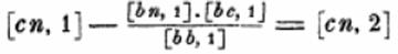
When Gauss reduces this system to triangular form he uses constructions of the form
Symbols for determinants. See DETERMINANT on Words.
All the authors who produced notation for systems of equations produced notation for determinants. A great variety of notations are displayed by Muir and Cajori.
The use of a single vertical line on both sides of the entries seems to have introduced by Cayley writing in 1841: see Muir vol. 1 p. and Cajori vol. 2, p. 92.
The notation appears in the Cambridge Mathematical Journal, Vol. II (1841), p. 267-271, reprinted in Papers vol. 1, p.1. On p. 1 Cayley writes
By the early twentieth century the modern combination of bar lines and the aij symbols for elements are found in textbooks: see Bôcher's Introduction to Higher Algebra (1909) and Kowalewski's Einführung in die Determinantentheorie (1909).
Symbols for Matrices. See MATRIX on Words.
Determinants had been studied for well over a century and a half before the idea of a matrix appeared. Cayley wrote about matrices on several occasions without seeming to settle on a fixed notation.
In his "Mémoire sur les Hyperdéterminants" of 1846, Crelle, 50 p. 2 Cayley uses the double vertical line notation found in works from the 1930s.
In his most substantial work on matrices, "A Memoir on the Theory of Matrices" of 1855 (Papers, II, 475-96), Cayley does not use such nice notation. He writes (p. 475).
A set of quantities arranged in the form of a square, e.g.
Cayley explained the motivation for introducing matrices:
The notion of such a matrix arises naturally from an abbreviated notation for a set of linear equations, viz. the equations
Cayley's main interest was in powers of square matrices (below) and matrix polynomials. The big result in the 1855 paper is the CAYLEY-HAMILTON THEOREM. Cayley uses upper-case letters for matrices but there is nothing systematic about his notation.
Matrix algebra was rediscovered by Frobenius; see "Ueber lineare Substitutionen und bilineare Formen," J. reine angew. Math. Vol. 84 (1878) pp.1-63. The notation in this and in his later works was much more sophisticated than that used by Cayley.
The printing of Cayley's matrices always looks improvised but more permanent forms followed. Cajori (vol. 2, p. 103) writes that round parentheses were used for matrices by many, including Maxine Bôcher in 1909 in Introduction to Higher Algebra and G. Kowalewski in 1909 in Determinantentheorie (although Kowalewski also used double vertical lines and a single brace).
In the 1930s books on matrices written in English started to appear. The two leading ones were C. C. MacDuffee Theory of Matrices, Springer (1933) and J. H. M. Wedderburn Lectures on Matrices (1934). They both wrote matrices with double vertical lines as in
Matrix inverse. See INVERSE on Words.
In the "Memoir" Cayley describes the formation of powers of matrices including the inverse of the matrix: see Papers, I, 480.
Cayley used 1 for the identity matrix and 0 for the zero matrix. Both Wedderburn Lectures on Matrices (1934, p. 8) and MacDuffee use I and O.
Transpose. See TRANSPOSE on Words.
MacDuffee Theory of Matrices (1933, p. 5) reports, "Many different notations for the transpose have been used, as A', Ā, Ă, A*, A1, 1A." His preference is for AT: "The present notation is in keeping with a systematic notation which, it is hoped, may find favour." Wedderburn Lectures on Matrices (1934, p. 8) writes A' for what he calls the transverse.
Kronecker product. See KRONECKER PRODUCT on Words.
F.D. Murnaghan Theory of Group Representations (1938, p. 68) writes A X B for the Kronecker product. The same symbols is used by Wedderburn Lectures on Matrices (1934, p. 74) although he uses the term direct product as does MacDuffee The Theory of Matrices, (1933, p. 81). MacDuffee writes A . X B although the dot is not printed quite so high.
Generalized inverse. See GENERALIZED INVERSE on Words.
The generalized inverse of A is written as A† by R. Penrose in "A Generalized Inverse for Matrices," Proc. Cambridge Philos. Soc., 51, (1955), 406-413. However the symbol A- quickly became popular; see e.g. C. R. Rao (1962) Note on a Generalized Inverse of a Matrix with Applications to Problems in Mathematical Statistics, Journal of the Royal Statistical Society B, 24, 152-158.
Symbols for Vectors. See VECTOR on Words.
Vector notation and indeed the idea of a vector developed independently of matrix ideas; the vector development had more to do with generalising complex numbers. M. J. Crowe A History of Vector Analysis (1967/87) describes the nineteenth century work of Hamilton, Grassmann and Gibbs.
Of these Gibbs seems to have had the greatest influence on the notation, but not through his own writing. His vector analysis became widely known through E. B. Wilson's Vector Analysis: A Text Book for the Use of Students of Mathematics and Physics Founded upon the Lectures of J. Willard Gibbs (1901).
Many symbols have come and gone: e.g. it is now standard to use the ordinary equals sign to represent equality between vectors but Cajori (pp. 133-4) shows earlier writers reluctant to do this and using a variety of equals-like symbols.
Vectors and scalars
In his Elements of Vector Analysis (1881) Gibbs writes, "we shall use small Greek letters to denote vectors and the small English letters to denote scalars." (Scientific Papers, 2, p. 17).
One of the innovations in Wilson's book was very influential, the use of Clarendon (bold) type for vectors and ordinary type for scalars. E.g. "Thus if A be the vector and x the scalar, the product is denoted by x A or A x."
Wilson used the bold/ordinary pair to representing a vector and its length: if A is a vector, then A is the scalar denoting its length. Later writers used the bold/ordinary type possibility to mark other distinctions. In Hermann Weyl's Raum, Zeit, Materie (Space, Time, Matter, 4th edition 1921) the bold type x represents the vector but the ordinary type xi represents a component of the vector. German writers also used old German (Gothic) characters to represent vectors and modern script for components: see Courant and Hilbert's Methoden der Mathematischen Physik (1924).
Following Hamilton's example, Wilson writes the "3 fundamental unit vectors" as i, j and k. Hamilton was extending the notation for complex numbers. The corresponding notation in Weyl's Raum, Zeit, Materie (for n-dimensional spaces) is e1 ,.., en .
Associated symbols
Scalar product and inner product. See INNER PRODUCT and DOT PRODUCT on Words.
In the Elements (1881) Gibbs wrote α.β for what he called the direct product of the vectors α and β.
In Vector Analysis Wilson wrote A∙B. The notation inspired the alternative term for the direct product, the dot product
Other authors used symbols resembling Gauss's symbol: see above. Cajori (p. 135) reports that (u,v) was used in Henrici and Turner's Vectors and Rotors (1903). In his paper axiomatising HILBERT SPACE, "Allgemeine Eigenwerttheorie Hermitescher Funktionaloperatoren," Math. Ann. 102, (1929), 49-131, von Neumann used the symbol (f,g)
Vector product. See VECTOR PRODUCT on Words.
In the Elements (1881) Gibbs wrote α X β for what he called the skew product of the vectors α and β.
In Vector Analysis Wilson wrote the skew product as A X B. The notation inspired the term cross product. See CROSS PRODUCT.
Length or norm. See NORM
Wilson's use of ordinary type has been mentioned. The absolute value symbol of Weierstrass (see Function Symbols), or some modification of it, has often been used. The symbols |X| and ║φ║ both appear in Banach's "Sur les opérations dans les ensembles abstraits et leur application aux équations integrales", Fundamenta Mathematicae, 3, (1922) 133-181.
For the vector calculus symbols see the calculus page.
Matrix notation in least squares/regression.
For the past fifty years or so it has been common to write the REGRESSION model in matrix notation as
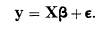
Such notation can be found in J. Durbin and G. S. Watson "Testing for Serial Correlation in Least Squares Regression: I," Biometrika, 37, (1950) and O. Kempthorne's Design and Analysis of Experiments (1952). Matrix notation was first used in the 1920s but the most noticed of the early contributions was a paper by Aitken, "On least squares and linear combinations of observations," Proc. Royal Soc. Edinburgh, 55, (1935), 42-48.
See also Regression and Matrix notation in Symbols in Probability & Statistics. The use of matrix theory in statistics is described by R. W. Farebrother "A. C. Aitken and the Consolidation of Matrix Theory," Linear Algebra and its Applications, 264, (1997), 3-12. For the earlier Gauss notation that was used in works on the combination of observations, or theory of errors, see above.